kz_filter项目解析(三)
今天看的主要是detrend.py这个文件的实现逻辑
我感觉前两天走的公式逻辑以及kz_filter代码逻辑还是有帮助的
背景足够熟悉,接下来无论是实现的场景还是设计的思路都能更加清楚
首先我看了一下代码的结果出图,在kzfilter-master\detrend*.png**里面
样例代码用的是input=9,也就是Tsuen wan城市
结果为
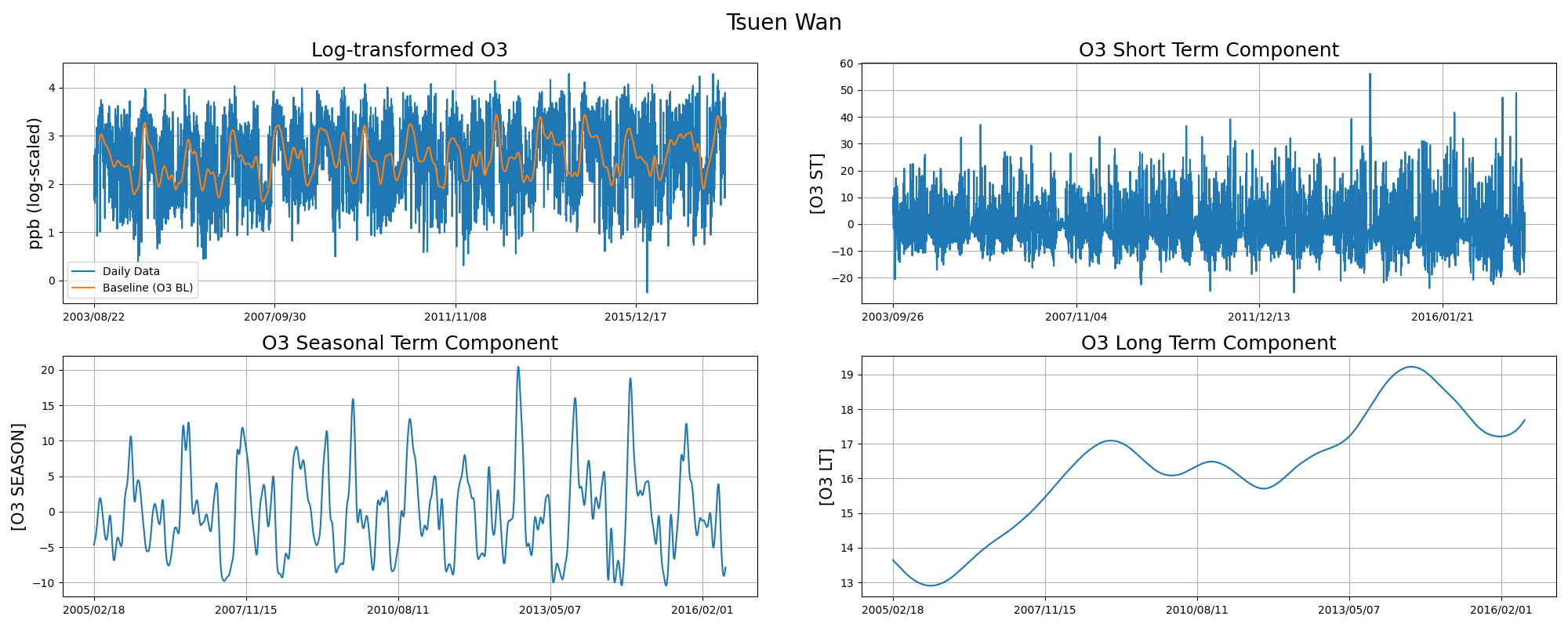
由结果推论,可得四个主要数据,分别为
- Log-transformed O3 (经log自然指数e转型后o3数据曲线)
- O3 Short Term Component (短期o3数据指数,)
- O3 Seasonal Term Component (季度o3数据指数)
- O3 Long Term Component (年度o3数据指数)
接下来我们走代码
- 分段走的话,第一步看文件处理,这里主要将不同地区数据存入file或者file1和file2中
1 | filelist = ['Eastern', 'Kwai Chung', 'Tung Chung', 'YL', 'Kwun Tong', 'Macau', 'Sha Tin', 'ShamShuiPo', 'Tap Mun', |
下一步是数据预处理的读取过程,这一步不需要多说
1
2
3
4
5
6
7
8
9
10
11
12
13
14
15
16
17
18
19
20
21
22
23
24
25
26
27
28
29
30
31
32
33def detrend(file):
hours = 24
timestamp = []
height = []
o3 = []
source = []
status = []
details = []
delete_index = []
with open(file) as infile:
# 读取当前o3数据文件
reader = csv.reader(infile)
# 遍历往时间数组,o3值数组,状态数组填值
for rows, value in enumerate(reader):
if rows > 3:
timestamp.append(value[0])
height.append(float(value[1]))
o3.append(float(value[2]))
source.append(value[3])
status.append(float(value[4]))
details.append(float(value[5]))
if input > 3:
with open(file2) as infile:
reader = csv.reader(infile)
# 遍历往时间数组,o3值数组,状态数组填值
for rows, value in enumerate(reader):
if rows > 3:
timestamp.append(value[0])
height.append(float(value[1]))
o3.append(float(value[2]))
source.append(value[3])
status.append(float(value[4]))
details.append(float(value[5]))接下来将存放的数据进行进一步处理,主要用于截取所需时间段的数据,并精简数据量(每天只取一个小时的数据作为标志数据),具体请看对应行注释
1
2
3
4
5
6
7
8
9
10
11
12
13
14
15
16
17
18
19
20
21
22
23
24
25
26
27
28
29
30
31
32
33
34
35
36# 如果是Macau数据,只统计在2013-2015年的数据
if input == 5:
timestamp = timestamp[:-17543]
o3 = o3[:-17543]
# Tsuen Wan: Delete from 2003/08/19 (2003/02/12 [973] ~ 2003/08/19 [5574])
if input == 9:
o3 = o3[5574:]
timestamp = timestamp[5574:]
numberofelements = len(timestamp) # 157800
# 数据都是一小时取一次,所以数组的长度等于小时数,计算后可得天数
numberofday = int(numberofelements / hours) # 6575 days
daily_timestamp = []
# 这一个过程是确定一天只取最后一小时数据,返回daily_timestamp数组
for i in range(numberofelements):
if i % 24 == 23:
today = timestamp[i].split()[0]
daily_timestamp.append(today)
print(daily_timestamp)
for i in range(len(timestamp)):
if o3[i] < 0:
delete_index.append(i)
print(numberofday, "days")
# delete_index是取出数据值小于0的非法值
print("Delete:", delete_index)
# findPositive方法可以取非法值前后的各第一个正常值,取其平均再存到o3数据列表中
for j in range(len(delete_index)):
o3[delete_index[j]] = functions.findPositive(o3, delete_index[j])
print("First Row:", timestamp[0], height[0], o3[0], source[0], status[0], details[0])
# 打印o3数据平均值
print("Mean", round(mean(o3), 4))
# 取选中数据的每天平均值存放到数组里
daily = functions.Daily(o3)
x = np.array(daily)
# t = np.arange(0, numberofday, dt)
t = np.array(daily_timestamp)至此准备工作完成,进行第一幅月度log曲线图(以此为例,后面类似)
首先定义数据,对应到公式里面的m,k,t
1
2
3
4
5
6
7
# 以月度为周期统计o3数据变化值
m = 29
k = 3
# 取选中数据的每天平均值存放到数组里
daily = np.array(daily)
# 生成daily的自然对数底数e(2.71828)对应的log值数组,这是为了使得减小数据的纵向差值
daily = np.log(daily)之后把数据带入公式中并append到结果集合
1
2
3
4
5
6
7
8
9
# 得到kz_filter之后的结果集合
o3_bl = kz_filter(daily, m, k)
# Adjust time
# 这里的w是我们之前在公式推导中所需要用到的遍历范围值
w = int(k * (m - 1) / 2)
# daily_timestamp2可以把数据从daily_timestamp得到-w到w的区间值
daily_timestamp2 = daily_timestamp[w:-w]
# 将月度数据放进subplot_matrix结果集合中
subplot_matrix.append([daily_timestamp, daily, daily_timestamp2, o3_bl])将几组数据处理完成后,进行图像绘制工作,这一部分逻辑比较简单,就不过多赘述了
1
2
3
4
5
6
7
8
9
10
11
12
13
14
15
16
17
18
19
20
21
22
23
24
25
26
27
28
29
30
detrend(file)
# Subplot
fig = plt.figure(figsize=(20, 8))
plt.suptitle(filelist[input], fontsize=20)
for count in range(len(subplot_matrix)):
data = subplot_matrix[count]
ax = plt.subplot(2, 2, count + 1)
ax.grid(True)
if count == 0:
ax.plot(data[0], data[1], label='Daily Data')
ax.plot(data[2], data[3], label='Baseline (O3 BL)')
ax.legend(loc='best')
else:
ax.plot(data[0], data[1])
ax.xaxis.set_major_locator(plt.MaxNLocator(5)) # Set Maximum number of x-axis values to show
if count == 0:
titles = 'Log-transformed O3'
plt.ylabel("ppb (log-scaled)", fontsize=15)
elif count == 1:
titles = 'O3 Short Term Component'
plt.ylabel("[O3 ST]", fontsize=15)
elif count == 2:
titles = 'O3 Seasonal Term Component'
plt.ylabel("[O3 SEASON]", fontsize=15)
else:
titles = 'O3 Long Term Component'
plt.ylabel("[O3 LT]", fontsize=15)
plt.title(titles, fontsize=18)
plt.tight_layout()
plt.subplots_adjust(wspace=0.15, top=0.9)